Numerical Methods for Solving Nonlinear Equations
Numerical Methods for Solving Non-linear Equations
Suppose you are trying to solve the equation:
$$sin(x) = 0.5 x$$
Can you do this algebraically?
No - but there are several variations on a theme of trial and error which we can use
Interval Bisection
First change your equation into a function for which you wish to find the roots
$$f(x) = sin(x) - 0.5 x$$
and solve
$$f(x) = 0$$
Plot the function $f(x)$ in excel
Define the function $f$ in VBA
Set up a start value and an end value for $x$ in excel
Draw a table of $x$ against $f(x)$ in Excel from start value to end value
Plot the graph
Now all we need to do to find out the root is to keep changing the start_value and end_value until we are as close in accuracy as we wish to be
Set the start_value to just before the root and set the end_value to just after the root. The graph should automatically redraw
Repeat process until to are happy you are close enough to the root and you have found the solution to the equation
Write a function, using the interval bisection method, which takes a start_value, an end_value and the name of a function as arguments and returns a root of the function between the start and end value
Flowchart for Interval Bisection

Improving your code
It is a good idea to check if a root does lie between the two initial values at all. If it does not then you can use CVErr to return an error code like so
You will also need to use the Sgn function to test the sign of the values calculated. Sgn returns -1,0 or 1 depending on the values of its argument.
If you wish to jump out of the function for some reason (most likely error handling) then you can use the following line of code
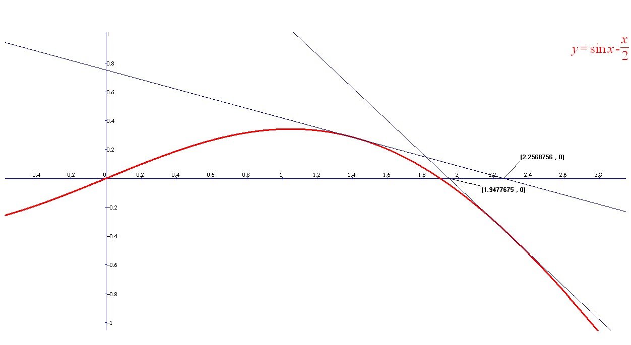
Newton Rhapson
The Newton Rhapson method has the advantage of being much faster as it uses the gradient of the graph to find the next approximation
The method is as follows:
- Start by guessing where the root is: this guess is $x_0$
- Find the next estimate with the formula:
$$x_{i+1} = x_i - \frac{F(x_i)}{F'(x_i)} , i=0,1,2,...,$$
- Stop when $|x_{n+1}-x_n|\approx 0$
You can see from the graph below how each tangent gets you closer and closer to the root
Write a function which takes an initial estimate, the name of a function and the name of the derivative of the function and returns the root found by Newton Rhapson.
Improving your code
Can you adapt the code so that it can handle situation where $F'(x) \approx 0$?
Can you adapt your code so it can handle getting stuck in an infinite loop?
Can you adapt your code to be sure it has found the smallest root as opposed to another root?
How might you change this function so it could handle not being sent the derivative of the function?
Mathematical Methods for Solving Differential Equations
Mathematical Methods for solving Differential Equations
In this chapter we will consider different methods of solving differential equations. By considering an equation to which we can calculate the answer exactly (the basic compound interest equation) we will be able to show the different levels of accuracy of the different methods.
So we are going to try and solve $\frac{dy}{dx}=ky$
Euler Method
The equation $\frac{dy}{dx}=ky$ is basically saying that the bigger $y$ is, the greater the rate at which it increases
A very simple way of trying to solve this equation is:
- take our starting value of $y$: $y_0$
- calculate $\frac{dy}{dx}$ at this point in time $t_0$ and then
- add our value of $\frac{dy}{dx}$ at $t_0$ to $y_0$
- to give us the value of $y$ at the next point in time i.e. $y_1$
If $x_1 - x_0$ is anything other than $1$ then we must adjust by this also. So our formula is:
$$y_{n+1} = y_n + (x_{n+1}-x_n) \times \left(\frac{dy}{dx}\right)_{n}$$
For $y_0=10$ and $k=0.4$:
Calculate $y_5$ using step sizes of:5, 1, 0.1 and 0.01
Compare your answers with the analytical answer $y=y_0 \times e^{kx}$
The problem with the Euler method is that as we move towards the end of the interval we are still using the derivative from the start of the interval and so we are losing accuracy
Rung Kutta
The solution to the loss of accuracy is to take the derivative at the end of the interval and then use this to recalculate the step change over the interval. Clearly this changes the vaue at the end of the interval which changes the derivative at the end of the interval. Much algebra ensues and the resulting 4th order Runge-Kutta equations, for the a problem defined as: $\dot{y}=f(x,y)$, $y(x_0)=y_0$ are as follows:
$y_{n+1}=y_n+\frac{h}{6}\left(k_1+2k_2+2k_3+k_4\right)$
$x_{n+1}=x_n+h$, for choice of interval $h$
Where:
$k_1=f(t_n, y_n)$
$k_2=f(t_n+\frac{h}{2}, y_n+\frac{h}{2}k_1)$
$k_3=f(t_n+\frac{h}{2}, y_n+\frac{h}{2}k_2)$
$k_4=f(t_n+h, y_n+hk_3)$
Now repeat the compound interest exercise from above using the Runge-Kutta method
For $y_0=10$ and $k=0.4$:
Calculate $y_5$ using step sizes ($h$) of:5, 1, 0.1 and 0.01
Compare your answers with the analytical answer $y=y_0 \times e^{kx}$ and with the answers under the Euler method
Quadratures
Quadratures
Introduction
A quadrature is just a name we use to describe methods of numerical integration
In this chapter we will look at some simple methods such as the trapezium rule, which you will already be familiar with and then we will consider some more sophisticated developments, such as Simpson's and Boole's rule, which interpolate function points with polynomials of increasing degree
Finally we will look at Gaussian quadratures where the assumption of evenly spaced abscissa points is dropped and a more general form of quadrature is developed which can produce remarkably accurate results with relatively little calculation
Very basic quadrature methods
The most basic form of numerical integration is called the left point rule: In this case we simply divide the function into intervals of width $\Delta x$ and then add up the area of the rectangles width: $\Delta x$ and height: $f(x_i)$, where $x_i$ is the value of $x$ at the left of the interval
This gives: $\int_{a}^{b}f(x) dx \approx \Delta x \times \left(f(x_0)+f(x_1)+...+f(x_{n-1})\right)$
where $a=x_0$, $b=x_n$ and the $x_i$s are evenly spaced across the interval.
The right point rule and the mid-point rule follow by analogy
Clearly these methods are very primitive and it is easy to improve on them
The Trapezium Rule
The trapezium rule represents the first level of sophistication in the numerical calculation of integrals
consider the problem of how to calculate the area under the curve: $y=e^{-x} \times sin x$ between $0$ and $\pi$
The following graph shows how we could use a series of trapeziums to estimate this integral

We can easily see that the area under the trapeziums reduces to:
$A=\frac{\pi}{8} \times \left(f(0) + 2f(\frac{\pi}{4}) + 2f(\frac{\pi}{2}) + 2f(\frac{3\pi}{4}) + f(\pi) \right)$
So more generally the trapezium rule is given by:
$\int_{a}^{b} f(x) dx \approx \frac{\Delta x}{2} \times \left(f(x_0)+2f(x_1)+2f(x_2)+...+2f(x_{n-1})+f(x_{n})\right)$
Write a VBA routine to approximate the integral of a general function between abscissas $a$ and $b$ with any given number of intervals using the trapezium rule
Approximate the area under $y=e^{-x} \times sin x$ between $0$ and $\pi$ using 4, 12 and 120 intervals
Simpson's Rule
Suppose instead of fitting straight line segments to our function we attempt to find a better fit by fitting quadratic segments
Look at the same function below (grey) with two black quadratics fitted to the first three and last three calculated function points
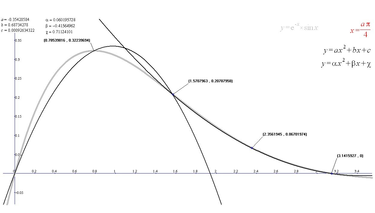
By considering a function $f$ on the interval $[-\theta, \theta ]$ and using abscissa points $-\theta$, $0$ and $\theta$, calculate the quadratic which will interpolate the three points
Using basic calculus, calculate the area under this quadratic on the interval $[-\theta, \theta ]$ as a function of $\theta$, $f(-\theta)$, $f(0)$ and $f(\theta)$
This leads us to Simpson's Rule which is stated generally as:
$\int_{a}^{b} f(x) dx \approx \frac{\Delta x}{3} \times \left(f(x_0)+4f(x_1)+2f(x_2)+4f(x_3)+...+2f(x_{n-2})+4f(x_{n-1})+f(x_{n})\right)$
Write a VBA routine to approximate the integral of a general function between abscissas $a$ and $b$ with any given number of intervals using Simpson's Rule
Approximate the area under $y=e^{-x} \times sin x$ between $0$ and $\pi$ using 4, 12 and 120 intervals using Simpson's Rule (2,6 and 60 quadratic segments)
Simpson's three eighths Rule
The next level is to fit cubic segments
Look at the same function again (grey) with the red cubic fitted to four calculated function points
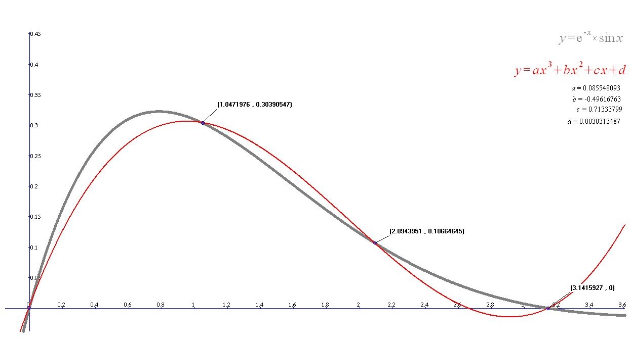
The principles are exactly the same but the algebra is a bit more complicated, so Simpson's 3/8ths Rule over a $3\Delta x$ interval can be expressed as:
$\int_{a}^{b} f(x) dx \approx \frac{3\Delta x}{8} \times \left(f(x_0)+3f(x_1)+3f(x_2)+f(x_3)\right)$
Write a single VBA routine to approximate the integral of a general function between abscissas $a$ and $b$ with any given number of intervals and allowing the user to choose between the methods given so far
Approximate the area under $y=e^{-x} \times sin x$ between $0$ and $\pi$ using 3, 6, 12 and 120 intervals using Simpson's 3/8ths Rule
Boole's Rule
The next level is to fit quartic segments
This time the interpolating function is a quartic
The principles are again the same, so Boole's Rule over $4\Delta x$ interval can be expressed as:
$\int_{a}^{b} f(x) dx \approx \frac{\Delta x}{45} \times \left(14f(x_0)+64f(x_1)+24f(x_2)+64f(x_3)+14f(x_4)\right)$
Extend your VBA routine to include Boole's Rule
Approximate the area under $y=e^{-x} \times sin x$ between $0$ and $\pi$ using 4, 12 and 120 intervals using Boole's Rule
Programming Extensions
There are a number of things you should now do to tidy up your routine
- Ensure the routine checks for an appropriate number of intervals for each integration method
- You could splice different methods where $n$ does not fit
- You could include an option to leave out $n$ and let the routine try different values until some convergence criterion is reached
Monte Carlo Methods
Monte Carlo Methods
A Monte Carlo method is any method which uses thousands of randomly generated scenarios to calculate approximate probabilities or expected values
This is very useful in finance as many variables are unknown and have to be simulated with random variables.
The relationships are also often very complicated and so closed form solutions are often not feasible.
The basic method is to model your random variables in VBA, then run the model thousands of times and then the probability of the 'positive' event is approximately the number of 'positive' results divided by the number of trials
Example 1
Draw a unit circle inside a square and use a Monte Carlo method to approximate the value of $\pi$
Example 2
On a chess board a knight starts in square 'A1'. It then moves randomly 20 times. What is the probability that it finishes in square 'A1'
Example 3
There are 10 red balls in bag 1, 10 green balls in bag 2 and 10 blue balls in bag 3. If you take one ball from bag 1 and put in it bag 2 and then take 1 ball from bag 2 and put it in bag 3 and then take one ball from bag 3 and put it in bag 1. Then you repeat this task 5 times, what is the probability that the last ball (the 15th) is blue